 TSampledSurface3D divides a 3D surface into small units called shards. Shards are small portions of a 3D surface that are defined by discrete points. The shards can be any shape and size.
Fractal surfaces, data that is digitized or scanned from realworld sources, reconstructions like volumetric CAT scans, and shapes approximated from other computations (like fluid flow) are all examples of surfaces that can be divided into shards.
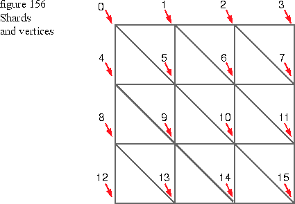
Figure 156
shows a square surface broken into triangular shards. The numbers in the figure correspond to the vertices of the shards. Each vertex of each shard contains information for normals, colors, and texture map indices to give you detailed control over the appearance of the discretized data when it is rendered.

Class architecture
TSampledSurface3D and its related classes are abstract and require that you design and implement their functionality to specify the discrete points that define the shards. TSampledSurface3D is based on a 3D surface geometry and does not descend from MGraphic3D.
Figure 157 shows TSampledSurface3D and its related classes. All of these classes are abstract base classes, and all of their functions are pure virtual. These classes guide you in creating your own TSampledSurface3D implementation.

The next two sections each present an example. The first example is a 3D digitizer, and the second example is a finite element mesh rendering.
Example data from
a 3D digitizer
The data from a 3D rangefinder digitizer is stored as an array of depth values that represent the z coordinates for the rendered surface. The field of the range finder is already known and is divided into equal steps. As shown in Figure 158, the data from the range finder are the z coordinates, and the x and y coordinates are implied.

The rangefinder data is shown in Figure 159.

TShardChunkIterator::CopyVertexInfo() gets the first 10,000 data points from the scanner, and supplies the x and y coordinates. Since one million is a large number of data points, for this example the data is used in 10 smaller chunks.
  Boolean
  TShardChunkIterator::CopyVertexInfo( TShadingInfoArray& data )
  {
      // fRawData is a 1,000,000 element array with the 1000 x 1000
      // collection of data from the scanner. fChunkCount keeps track of
      // how many times CopyVertexInfo has been called.

      if (fChunkCount == 10)
          return FALSE;                   // All data has been copied out

      for (i = 0; i < 100; i++)// 100 rows in this chunk
           for (j = 0; j < 1000; j++)     // 1000 items per row
           {
          data[i * 1000 + j] = kDefault;  // Set default color, etc.

          TGPoint3D * p = &data[i * 1000 + j].fPoint;

          p>fX = j;  // Generate implied X and Y
          p>fY = fChunkCount * 1000 + i

          p>fZ = fRawData[(fChunkCount * 1000 + i)*1000 + j];
          }
      fChunkCount++;
      return TRUE;
  }
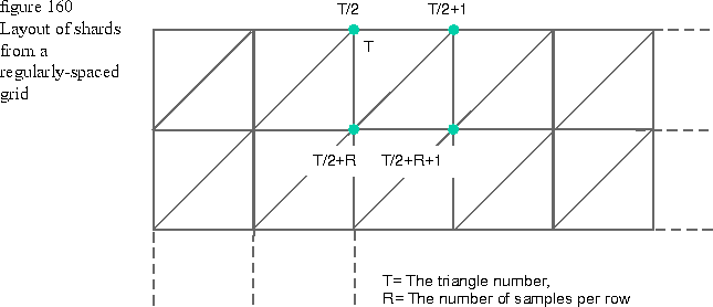
Next, create a shard iterator to generate the triangles for rendering the surface from the scanner data. The shard iterator generates indices into the vertex information that CopyVertexInfo function generated (only the topology for hooking the triangles up is required) using the numbering scheme shown in Figure 160. An implementation of TShardIterator::GetNextShard is also shown.

  TShardIterator::GetNextShard(  long& i0, long& i1, long& i2, Boolean& edge01vis,
                        Boolean& edge12vis, Boolean& edge20vis )
  {
      // fShardNumber is the number of the shard generated.
      if (fShardNumber == 1000 * 100)
          return FALSE;               // All shard for this chunk generated

      if (even( fShardNumber ))
      {
          i0 = fShardNumber / 2;
          i1 = fShardNumber / 2 + 1000;
          i2 = fShardNumber / 2 + 1;
          // Show edge visibility, diagonal edges are not visible.
          edge01vis = TRUE; edge12vis = FALSE; edge20vis = TRUE;
      }
      else // odd # shard
      {
          i0 = fShardNumber / 2 + 1;
          i1 = fShardNumber / 2 + 1000;
          i2 = fShardNumber / 2 + 1000 +1;
          // Show edge visibility, diagonal edges are not visible.
          edge01vis = FALSE; edge12vis = TRUE; edge20vis = TRUE;
      }
      fShardNumber++;
      return TRUE;
  }
NOTE  The Boolean settings of the edge visibility cause the diagonal edges of the shards to be invisible if the surface is rendered as a wireframe. No clipping or backface culling of surfaces have been used.
Example finite element mesh rendering
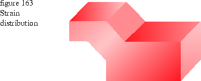
A finite element model (FEM) is created with 3D modelling software. Usually a part is designed to meet particular shape requirements, and then "meshed," or broken into shards by the FEM software. At the vertices of the shards, the FEM software calculates the amount of strain energy on the vertices. These strain energy estimations are usually converted into color gradients to give a graphical display of the strain on the part. A simple model might be a brace such as the one shown in Figure 161.

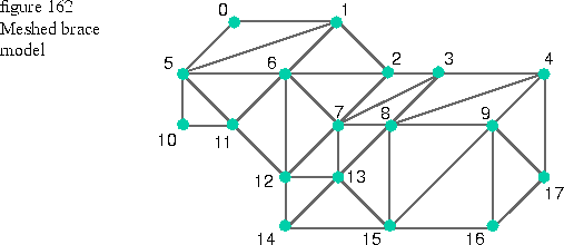
The meshed model generated by the FEM software looks something like the model in Figure 162. In addition to (x, y, z) geometric position information, each of the numbered vertices has a value to represent the strain energy at that point.

The model generated by the FEM software might be stored as a list of vertices (like those numbered in the figure above), and a list of triangular shards formed by those vertices (for example, (0, 5, 1), (1, 5, 6), (5, 10, 11), (1, 6, 2), and so on) where the numbers in parenthesis refer to the indices of the vertices.
The CopyVertexInfo routine is implemented as follows (it assumes that the FEM data is loaded elsewhere).
  Boolean
  TShardChunkIterator::CopyVertexInfo( TShadingInfoArray& data )
  {
      for (i = 0; i < NumberFEMVertices; i++)
      {
          data[i].fPoint.fX = FEMdataXCoordinate[i];
          data[i].fPoint.fY = FEMdataYCoordinate[i];
          data[i].fPoint.fZ = FEMdataZCoordinate[i];

          // Set the color according to the strain energy at the
          // vertex. Energy to Color performs some userdefined
          // mapping, perhaps via a lookup table.

          data.fBaseColor[i] = EnergyToColor( FEMdataStrain[i] );
      }

      // This assumes all data is processed in one step. For large data sets,
      // this can be broken into multiple calls, like in the first example.
      return FALSE;
  }
  TShardIterator::GetNextShard(  long& i0, long& i1, long& i2,
                        Boolean& edge01vis,
                        Boolean& edge12vis,
                        Boolean& edge20vis )
  {
      if (fNumberOfShards > FEMdataNumberOfShards)
          return FALSE;                   // All shards rendered

      i0 = FEMdataV0index[ fNumberOfShards ];
      i1 = FEMdataV1index[ fNumberOfShards ];
      i2 = FEMdataV2index[ fNumberOfShards ];

      // Edge visibility may or may not be useful
      edge01vis = FALSE; edge12vis = FALSE; edge20vis = FALSE;

      fNumberOfShards++;
      return TRUE;
  }

In addition to strain energy, variables such as temperature distribution can be displayed with this technique, which is commonly used for data sets generated by many scientific visualization applications.